Seq2seq Model with Attention

Digested and reproduced from Visualizing A Neural Machine Translation Model by Jay Alammar.
Table of Contents
Sequence-to-sequence models are deep learning models that have achieved a lot of success in tasks like machine translation, text summarization, and image captioning. Google Translate started using such a model in production in late 2016. These models are explained in the two pioneering papers (Sutskever et al., 2014, Cho et al., 2014).
A sequence-to-sequence model is a model that takes a sequence of items (words, letters, features of an images…etc) and outputs another sequence of items.
In neural machine translation, a sequence is a series of words, processed one after another. The output is, likewise, a series of words:
1. Architecture of Seq2seq
The model is composed of an encoder and a decoder. The encoder processes each item in the input sequence and compiles the information into a vector (called the context ). After processing the input sequence, the encoder sends the context over to the decoder , which produces the output sequence item by item.
The same applies in the case of machine translation.
RNN (recurrent neural network) is shown as an illustration here to be the model of both encoder and decoder (Be sure to check out Luis Serrano’s A friendly introduction to Recurrent Neural Networks for an intro to RNNs).
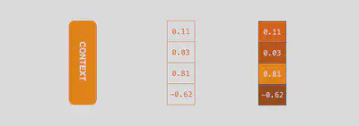
You can set the size of the context vector when you set up your model. It is basically the number of hidden units in the encoder RNN. These visualizations show a vector of size 4, but in real world applications the context vector would be of a size like 256, 512, or 1024.
By design, a RNN takes two inputs at each time step: an input (in the case of the encoder, one word from the input sentence), and a hidden state. The word, however, needs to be represented by a vector. To transform a word into a vector, we turn to the class of methods called “word embedding” algorithms. These turn words into vector spaces that capture a lot of the meaning/semantic information of the words (e.g. king - man + woman = queen).
 or train our own embedding on our dataset. Embedding vectors of size 200 or 300 are typical, we're showing a vector of size four for simplicity.](/post/attention/embedding_hue52ea6887e4ffd78961218df5eff4111_41024_4caff9934379c54892ef9e2a484b83fd.webp)
Now that we’ve introduced our main vectors/tensors, let’s recap the mechanics of an RNN and establish a visual language to describe these models:
The next RNN step takes the second input vector and hidden state #1 to create the output of that time step. Later in the post, we’ll use an animation like this to describe the vectors inside a neural machine translation model.
In the following visualization, each pulse for the encoder or decoder is that RNN processing its inputs and generating an output for that time step. Since the encoder and decoder are both RNNs, each time step one of the RNNs does some processing, it updates its hidden state based on its inputs and previous inputs it has seen.
Let’s look at the hidden states for the encoder. Notice how the last hidden state is actually the context we pass along to the decoder.
The decoder also maintains a hidden states that it passes from one time step to the next. We just didn’t visualize it in this graphic because we’re concerned with the major parts of the model for now.
Let’s now look at another way to visualize a sequence-to-sequence model. This animation will make it easier to understand the static graphics that describe these models. This is called an “unrolled” view where instead of showing the one decoder, we show a copy of it for each time step. This way we can look at the inputs and outputs of each time step.
2. Attention Mechanism
Attention is a generalized pooling method with. The core component in the attention mechanism is the attention layer, or called attention for simplicity. An input of the attention layer is called a query. For a query, attention returns an o bias alignment over inputsutput based on the memory — a set of key-value pairs encoded in the attention layer. To be more specific, assume that the memory contains $n$ key-value pairs, $(k_1, v_1), \cdots, (k_n, v_n)$ with $\mathbf{k}\in{ \mathbb{R}^{d_k}}, \mathbf{v}\in{ \mathbb{R}^{d_v}}$. Given a query $\mathbf{q}\in \mathbb{R}^{d_q}$, the attention layer returns an output $\mathbf{o}\in{ \mathbb{R}^{d_v}} $ with the same shape as the value.
Pros of using attention:
- With attention, Seq2seq does not forget the source input.
- With attention, the decoder knows where to focus.
The context vector turned out to be a bottleneck for these types of models. It made it challenging for the models to deal with long sentences. A solution was proposed in Bahdanau et al., 2014 and Luong et al., 2015. These papers introduced and refined a technique called “Attention”, which highly improved the quality of machine translation systems. Attention allows the model to focus on the relevant parts of the input sequence as needed.
Let’s continue looking at attention models at this high level of abstraction. An attention model differs from a classic sequence-to-sequence model in two main ways:
First, the encoder passes a lot more data to the decoder. Instead of passing the last hidden state of the encoding stage, the encoder passes all the hidden states to the decoder:
Second, an attention decoder does an extra step before producing its output. In order to focus on the parts of the input that are relevant to this decoding time step, the decoder does the following:
- Look at the set of encoder hidden states it received – each encoder hidden states is most associated with a certain word in the input sentence
- Give each hidden states a score (let’s ignore how the scoring is done for now)
- Multiply each hidden states by its softmaxed score, thus amplifying hidden states with high scores, and drowning out hidden states with low scores
This scoring exercise is done at each time step on the decoder side.
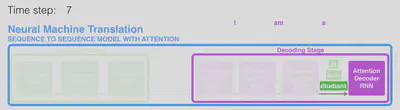
Let us now bring the whole thing together in the following visualization and look at how the attention process works:
- The attention decoder RNN takes in the embedding of the <END> token, and an initial decoder hidden state.
- The RNN processes its inputs, producing an output and a new hidden state vector (h4). The output is discarded.
- Attention Step: We use the encoder hidden states and the h4 vector to calculate a context vector (C4) for this time step.
- We concatenate h4 and C4 into one vector.
- We pass this vector through a feedforward neural network (one trained jointly with the model).
- The output of the feedforward neural networks indicates the output word of this time step.
- Repeat for the next time steps
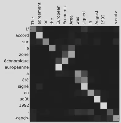
This is another way to look at which part of the input sentence we’re paying attention to at each decoding step:
Note that the model isn’t just mindless aligning the first word at the output with the first word from the input. It actually learned from the training phase how to align words in that language pair (French and English in our example). An example for how precise this mechanism can be comes from the attention papers listed above:
You can check TensorFlow’s Neural Machine Translation (seq2seq) Tutorial.