You only look once (YOLO) -- (1)

You Only Look Once (YOLO) is an object detection system targeted for real-time processing. There are three versions of YOLO: YOLO, YOLOv2 (and YOLO9000) and YOLOv3. For this article, we mainly focus on YOLO first stage.

1. Introduction

The target is to find out the bounding box (rectangular boundary frame) of all the objects in the picture and meanwhile judge the categories of them, where left top coordinate denoted by $(x,y)$, as well as the width and height of the rectangle bounding box by $(w,h)$.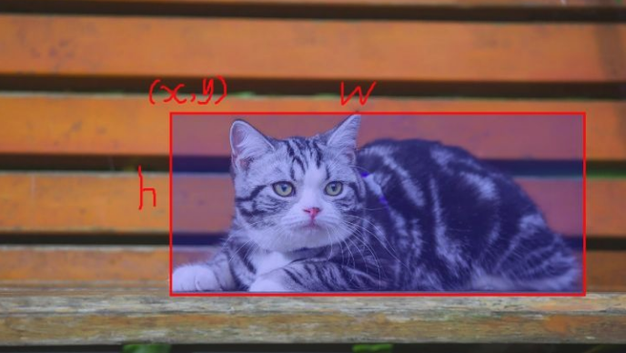

The challenge here is that we have unknown number of objects, so the output dimension is not fixed.

2. Grid Cell

The idea of YOLO is to output a fixed number of dimension which is big enough to contain all the objects. We crop the original picture and divide it into an $S\times S$ grid. Each grid cell predicts only one object. For example, the red grid cell tries to predict the “dog” object whose center falls inside that grid cell.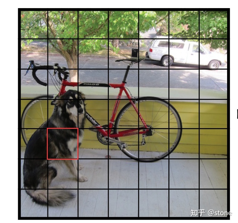

Each grid cell predicts a fixed number of boundary boxes. In the next example, the yellow grid cell makes two boundary box predictions (blue boxes) to locate where the person is.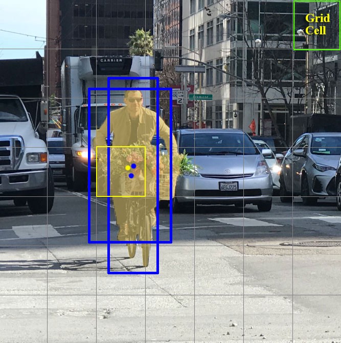

For each grid cell,

• it predicts B boundary boxes and each box has a box confidence score,
• it detects one object only regardless of the number of boxes B,
• it predicts C conditional class probabilities.

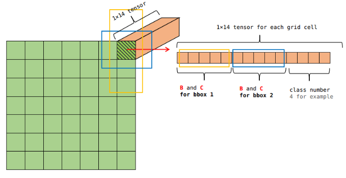
For example we can use $7\times 7$ grids ($S\times S$), 2 boundary boxes (B) with 1 corresponding confidence score and 4 coordinates ($w,h,x,y$), as well as 4 classes (C), which makes up for $1\times 14$ tensor.

3. Network Design

YOLO has 24 convolutional layers followed by 2 fully connected layers (FC). Some convolution layers use $1\times 1$ reduction layers to reduce the depth of feature maps. For the last convolution layer, the output is a tensor with shape $(7,7,1024). Then tensor is flattened, and finally output $7\times 7 \times 30$ parameters (if 20 classes and 2 bboxes predictions per grid cell) through linear regression.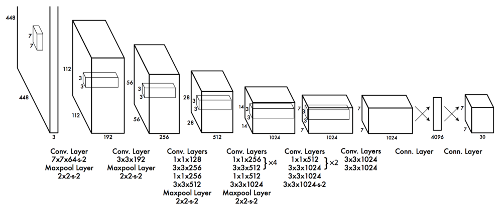

4. Loss Fuction

YOLO uses sum-squared error between predictions (the one with highest IoU) and ground truth to calculate loss. The loss function composes of:

• the classification loss.
• the localization loss.
• the confidence loss (the objectness of the box).

Classification loss

$$ \sum_{i=0}^{S^2} \mathbf{1}_i^{obj} \cdot{ \sum _{cc\in{classes}} \left( p _{i}(cc) - \hat{p} _i(cc) \right)^2} $$ where $\mathbf{1}_i^{obj} = 1$ if an object appears in cell $i$, otherwise 0;

$\hat{p} _i(cc)$ denotes the conditional class probability for class $cc$ in cell $i$.

Localization loss

\begin{aligned} \lambda _{coord} \sum _{i=0}^{S^2} \sum _{j=0}^{B} \mathbf{1} _{ij}^{obj} \left[ (x _i - \hat{x _i})^2 + (y _i - \hat{y} _i)^2 \right] \ + \lambda _{coord} \sum _{i=0}^{S^2} \sum _{j=0}^{B} \mathbf{1} _{ij}^{obj} \left[ (\sqrt{w _i} - \sqrt{\hat{w} _i} )^2 + (\sqrt{h _i} - \sqrt{\hat{h} _i} )^2 \right] \end{aligned}

where $\mathbf{1}_{ij}^{obj} = 1$ if the $j$th boundary box in cell $i$ is responsible for detecting object, otherwise 0;

$\lambda_{coord}$ increases the weight for the loss in the boundary box coordinates.

YOLO predicts the square root of bounding box width and height in order to differentiate large and small boxes. By setting $\lambda_{coord}$ (default: 5), we put more emphasis on the boundary box accuracy.

Confidence loss

If an object is detected in the box, the confidence loss is:

$$ \sum _{i=0}^{S^2} \sum _{j=0}^{B} \mathbf{1} _{ij}^{obj} \left( C _i - \hat{C} _i \right)^2 $$

where $\mathbf{1}_{ij}^{obj} = 1$ if the $j$th boundary box in cell $i$ is responsible for detecting the object, otherwise 0;

$\hat{C} _i$ is the box confidence score of the box $j$ in cell $i$.

However, if an object is not detected:

$$ \lambda _{backg} \sum _{i=0}^{S^2} \sum _{j=0}^{B} \mathbf{1} _{ij}^{backg} \left( C _i - \hat{C} _i \right)^2 $$

where $\mathbf{1} _{ij}^{backg} $ is the complement of $ \mathbf{1} _{ij}^{obj}$.

$\hat{C} _i$ is the box confidence score of the box $j$ in cell $i$.

$\lambda _{backg}$ weights down the loss when detecting background.

As most boxes do not contain any objects, we weight the loss down by a factor $\lambda _{backg}$ (default: 0.5) to balance the weight.

5. Inference: Non-maximal Suppression

Next, we multiply all these class scores with bounding box confidence and get class scores for different boudning boxes. So output is $7\times 7\times 2 = 98$.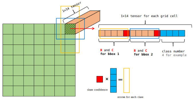

Then we set a threshold value of scores and sort them descendingly. Non-max supressing alogrithm is used to set score to zero for redundant boxes.

For example, dog score for bbox1 as 0.5 and bbox 2 as 0.3. We take an Intersection over Union (IOU) of these values and if the value is greater than 0.5, we will set the value for box2 as zero, otherwise continue to the next box.